4. Benchmarks
4.1. Experiment Settings
4.1.1. Algorithms
We have chosen the following five FL mechanisms which target different issues in the benchmarking:
FedSGD: FedSGD inherits the settings of large-batch synchronous SGD in data centers, and it is one of the most fundamental FL mechanisms.
FedAvg: FedAvg is a communication-efficient algorithm aggregating the parameters trained by multiple rounds of clients’ local training.
FedProx: FedProx targets the non-IID data problem and tries to improve the FedAvg using a regularization on the distance between the global and local models. We fix the regularization’s weight to 0.01 in the benchmark.
FedOpt: FedOpt proposed to use the adoptive optimization methods in FL. Three optimizations, including FedAdagrad, FedYogi, and FedAdam, are proposed. And we chose FedAdam in this paper’s benchmarking study.
4.1.2. Datasets
We have used five datasets in the experiments: MNIST, FEMNIST, CelebA, Sentiment140, and Shakespeare. One difference between the evaluation datasets used by FL and conventional machine learning is that the data samples are grouped by clients in FL. In our benchmarks, apart from the MNIST, all datasets contain the meta information grouping data samples according to the clients, e.g., the photos taken from the same celebrity are grouped together in CelebA, the words spoken by the same character are grouped together in Shakespeare. Most of the datasets contain a large number of clients, e.g., the Sentiment140 contains over 50,579 clients, which brings large efficiency overhead during the evaluation and requires significant computing resources, e.g., a cluster with 68 GPUs is used to emulate 1300 clients in existing work. To reduce the required sources and standardize the evaluation, we cut the datasets into different scales based on the number of clients and the number of train samples, including small, medium, large, and very large, which are presented in the following table:
| Datasets | Small | Medium | Large | Very Large |
|---|---|---|---|---|
| MNIST | 100 #C 300 #S 42.8% |
100 #C 700 #S 100% |
\ | \ |
| FEMNIST | 100 #C 237 #S 3% |
1000 #C 227 #S 28.6% |
3500 #C 226 #S 100% |
\ |
| CelebA | 100 #C 30 #S 1.5% |
1000 #C 30 #S 14.8% |
9343 #S 22 #S 100% |
\ |
| Sent140 | 100 #C 169#S 2.7% |
1000 #C 78#S 12.3% |
10000 #C 29 #S 45.8% |
50579 #C 13 #S 100% |
| Shakespeare | \ | 100 #C 489668 #S 11.6% |
1121 #C 4226158 #S 100% |
\ |
(Table Caption: Accelerate and standardize the evaluation by cutting the datasets into different scales. The information reported in the table is organized by: the number of clients (#C), the number of samples per client (#S), and the ratio of samples held by existing clients to the whole dataset.)
We use the median-scale datasets in all the experiments. Following the notation from previous work, we use \(B\), \(C\), and \(E\) to represent the clients’ local batch size, the ratio of selected clients for training and the clients’ local training passes. We set \(B=\infty, C=1.0\), and \(E=1\) for FedSGD on all datasets, and set \(B=128,C=0.1,E=10\) for the other methods on all datasets, except for \(B=1024\) on the Shakespeare dataset since it has a significant amount of training samples. Then we perform a fine-grained parameter tuning on the learning rate for each FL algorithm on each dataset, starting from 0.0001 to 3.
For datasets that are not collected in FL style (i.e., MNIST), we simulate the non-IID data by restricting the number of clients’ local image classes. For example, the experimental results of clients having 1 class of MNIST images are reported in the robustness benchmarks. For datasets collected in the FL manner (i.e., the samples are grouped by who generated them), we partition the data naturally based on the identity and randomly shuffle the data between clients to create an ideal IID data setting. To make the comparison close to the real-world setting, we use the non-IID data setting by default and only present the IID data results in the robustness evaluation.
4.1.3. Hardware
All the experiments run on a Linux server with Ubuntu 18.04 installed, Intel(R) i7-9700KF 8-core 3.7GHz CPU, 128GB RAM, 960G SSD storage. The hardware platform has 2 GPUs, however, we only use GPUs in the parameter tuning and use CPU for efficiency evaluation since most of the edge devices have no power GPUs. The containers are connected using the docker network using the bridge mode. In the efficiency evaluation, we config FedEval to limit each client can only use 1 CPU core and have a maximum of 8 clients running simultaneously since our CPU only has 8 cores, and we report the federated time consumption as the time evaluation results, which is introduced in our paper.
4.2. Radar Chart
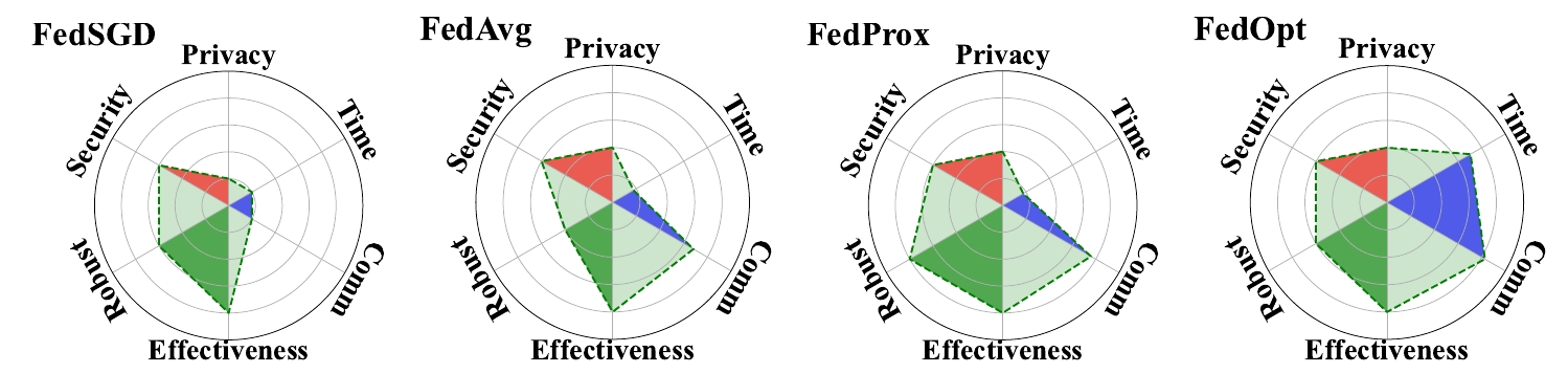
We have attempted to merge different evaluation measures into one radar chart for easy comparison. The challenge lies in quantifying different goals with disparate units and scales into a common range reasonably. We introduce the radar chart computation details next. Notably, the radar charts and computation method here represent our initial attempt; we will continue refining the charts in the future.
Efficiency score (quantitative): The efficiency score is the calculated through averaging the quantitative score of three sub-metrics, which are the communication rounds, communication amount, and the time consumption. For each of these sub-metrics, we choose one baseline model (i.e., FedSGD), score 1 point to the baseline model, and then compute the score of other methods through comparing to the baseline model. Specifically:
If the method A’s performance \(P_a\) (e.g., time consumption) is worse than the baseline model \(P_b\), then we give score \(e^{1-P_b/P_a}\) to A.
Otherwise, if method A’s performance \(P_a\) is better than the baseline model \(P_b\), denoting the best performance as \(\bar{P}\), then we give score \(1 + 4(P_b - P_a)/(P_b - \bar{P})\) to A. We set the best performance \(\bar{P}=0\) for time consumption, \(\bar{P}=1\) for communication rounds, and \(\bar{P}=0\) for communication amount.
Robustness score (quantitative):
Add \(3\) points if the non-IID performance disparity to IID model \(\le 1\%\).
Add \(2\) points if the non-IID performance disparity to IID model \(\le 3\%\).
Add \(1\) points if the non-IID performance disparity to IID model \(\le 5\%\).
Add \(1\) point if the stragglers are handled.
Add \(1\) point if the dropouts are handled.
Effectiveness score (quantitative):
If the model’s performance is better than the local model, we score according to the performance disparity to the central model. Score \(5 \sim 1\) if performance disparity to the central model is \(\le 1\%\), \(\le 3\%\), \(\le 5\%\), \(\le 10\%\), and \(\le 20\%\), respectively.
Score \(0\) if the performance is worse or equal to local model.
Security & Privacy score (qualitative):
For the privacy and security score, we temporarily use the qualitative score in the radar chart and will update the charts as well as the computation methods when more attack experiments are conducted. Briefly, we categorize the ability to defend against privacy and security attacks into different levels based on the amount of information transmitted between the server and clients.
For the ability to resist the privacy attack on the client side (if the clients send less information to the server, they have a stronger ability to defend against the data privacy attacks):
Score \(0\) if directly exchanging raw data.
Score \(1\) if the exchanged parameters are in plaintext and calculated from a single round of training.
Score \(2\) if the exchanged parameters are in plaintext and calculated from multiple rounds of training.
Score \(3\) if the exchanged parameters are protected by DP or the parameters are compressed.
Score \(4\) if the exchanged parameters are protected by secure aggregation.
Score \(5\) if the exchanged parameters are protected by homomorphic encryption.
For the ability to resist the model security attack on the server side (if the server receives more information, it has a stronger ability to defend against the model security attacks):
Score \(5\) if directly exchanging raw data, since the server can always make sure the model is training on the real dataset.
Score \(4\) if the exchanged parameters are in plaintext and calculated from a single round of training.
Score \(3\) if the exchanged parameters are in plaintext and calculated from multiple rounds of training.
Score \(2\) if the exchanged parameters are protected by DP or the parameters are compressed.
Score \(1\) if the exchanged parameters are protected by secure aggregation.
Score \(0\) if the exchanged parameters are protected by homomorphic encryption.